It’s that magical time of the year. Twinkling lights and sparkling ornaments delight the eyes; while gifts, laughter, family time, and steaming cups of glühwein warm the soul. Despite the winter chill, there’s a heartwarming joy in being part of the crowd, feasting these magical moments together.
It’s a job hazard, really – after wandering through Christmas markets for three days in a row, I couldn’t help but view everything through the lens of statistical analysis. Then it hit me. Why not explain statistical testing through the lovely examples of Christmas, to make them more enjoyable and easier to grasp. To everyone celebrating, I wish you a joyful Christmas filled love, laughter, and of course glühwein. Happy reading!
Let’s start with a little refresher on what statistical tests actually are. They are essential tools used to make inferences about the data. It’s a little like trying to predict the crowd size at the Christmas market – we make a hypothesis and test it to see if we’re right (or totally off!). We propose a statement – a hypothesis – about a research question, and test it using appropriate techniques – statistical tests – to admit or reject it. Choosing the right statistical test depends on the Data Type, distribution of the data, sample size and the nature of the hypothesis.
Data Types
There are four main data types which affects our decision on the chosen statistical test:
- Nominal: Categorical data with no inherent order. In other words, no ranking involved. Think of the stall types at a Christmas market, such as food, ornament, gift etc.
- Ordinal: Categorical data with a meaningful order. For example, the categories of visitor numbers across different Christmas markets, such as high, medium, low.
- Interval: Numeric data with equal intervals between values, but with no true zero. Think of the weather temperature, since 0°C does not mean the absence of the temperature, just a cold spot.
- Ratio: numeric data with true zero, where zero means the complete absence of the quantity. For example, the number of hot dogs sold or visitor number of the Christmas Market. If no one shows up, you’ve hit zero – and that’s a real zero.
Data Distribution
Data distribution refers to how values are spread or arranged across a dataset. Here’s a summary of key data distributions:
- Normal: the distribution is symmetric, with most data points clustering around the mean. It is also called bell curve.
- Skewed: the distribution is skewed, so one tail is longer than the other.
- Uniform: data points are spread evenly so all outcomes are equally likely.
- Bimodal: the distribution has two peaks, which may indicate two underlying groups.
- Exponential: the distribution has a high concentration of values at the lower end, but becomes sparse as values increase.
The data distribution is important to decide on whether parametric or non-parametric tests should be used. It’s like picking the right glühwein stall to get a delicious one— no one wants to wait in line at the wrong one!
Nature of Hypothesis
It refers to the type of claim or assertion being made about the data or population that is being tested in a Statistical Analysis. In general, hypotheses can be categorized into two: null hypothesis and alternative hypothesis.
- Null hypothesis: It suggests that there is no significant effect or relationship between variables in the population or data set being studied. Essentially, the null hypothesis assumes that any observed effect or difference is due to chance or random variation. For example: "The average spending per visitor is the same as it was last year."
- Alternative Hypothesis: It asserts that there is a significant effect, difference, or relationship in the data. It reflects the researcher’s theory or belief about the relationship between variables. For example: "The average spending per visitor at the Christmas market has changed compared to last year."
Sample Size and Error Types
Sample size refers to the number of observations or data points collected in a study. The sample size influences the ability to detect a true effect or relationship in the population and the precision of the estimates. The bigger the sample, the better the test. It’s like needing more snowflakes to make a perfect snowman – smaller samples give you less power, and larger ones help reduce errors.
There are two types of error:
- Type I error (False Positive): The probability of incorrectly rejecting the null hypothesis when it is true.
- Type II error (False Negative): The probability of failing to reject the null hypothesis when the alternative hypothesis is true.
Larger sample sizes reduce both types of errors, but they are particularly effective in reducing Type II errors.
Central Limit Theorem states that, regardless of the population distribution, the sampling distribution of the sample mean will be approximately normally distributed when the sample size is sufficiently large (typically n > 30).
Common Statistical Tests and When to Use Them
🎅 Tests for Means
One-Sample t-Test is used to compare the mean of a sample to a known value.
- Data Type: Interval or Ratio
- Data Distribution: Normal distribution
- Sample Size: Small or large (no minimum sample size requirement)
- Hypothesis: The average spending per visitor at a Christmas market different from last year’s average (€50).
Independent t-Test is used to compare means between two independent groups.
- Data Type: Interval or Ratio
- Data Distribution: Normal distribution
- Sample Size: Large (at least 30 sample per group)
- Hypothesis: The visitors spend more at markets in large cities versus small towns.
Paired t-Test is used to compare means of the same group before and after an event.
- Data Type: Interval or Ratio
- Data Distribution: Normal distribution.
- Sample Size: Small or large (no minimum sample size requirement)
- Hypothesis: The average glühwein consumed per hour increases after live music starts at the market.
🎁 Tests for Relationships
Pearson Correlation is used to measure the strength of a linear relationship between two continuous variables.
- Data Type: Interval or Ratio
- Data Distribution: Normal distribution
- Sample Size: Large (at least 30 sample per group)
- Hypothesis: There is a correlation between the number of stalls and total market revenue.
Chi-Square Test is used to assess relationships between categorical variables.
- Data Type: Nominal
- Data Distribution: Non-normal or unknown
- Sample Size: Large enough to avoid expected counts less than 5
- Hypothesis: Visitor preferences for ornament materials (wooden, plastic, metal, fabric) are independent of the city.
Spearman Rank Correlation is used to assess relationships between ordinal variables or non-linear data.
- Data Type: Ordinal or non-linear Interval/Ratio
- Data Distribution: Skewed or non-normal
- Sample Size: Small or large (no minimum sample size requirement)
- Hypothesis: There is a relationship between the number of Santa Claus flying performances and visitor ratings.
🎇 Tests for Proportions
Z-Test for Proportions is used to compare proportions in a sample to a known proportion.
- Data Type: Nominal
- Data Distribution: Normal distribution
- Sample Size: Large (at least 30 sample per group)
- Hypothesis: The proportion of stalls which sell candles higher this year compared to last year.
Chi-Square Test for Independence is used to compare proportions between two or more groups.
- Data Type: Nominal
- Data Distribution: Non-normal or unknown
- Sample Size: Large enough to avoid expected counts less than 5
- Hypothesis: The proportion of crepe stalls are similar with currywurst stalls across different cities in Germany.
🤶 Tests for Variances
F-Test is used to compare variances between two groups.
- Data Type: Interval or Ratio
- Data Distribution: Normal distribution
- Sample Size: Moderate or large (no strict minimum sample size)
- Hypothesis: The variances of total visitor numbers for Christmas markets in large and small cities are different.
Levene’s Test is used to test for equality of variances across groups.
- Data Type: Interval or Ratio
- Data Distribution: Non-normal or unknown
- Sample Size: Small or large (no strict minimum sample size)
- Hypothesis: The variances in the total amount sold at glühwein and hot cacao stalls are equal.
❄️ Tests for Multiple Groups
ANOVA (Analysis of Variance) is used to compare means across three or more groups.
- Data Type: Interval or Ratio
- Data Distribution: Normal distribution
- Sample Size: Large (at least 30 sample per group)
- Hypothesis: Average spending differs across Christmas markets in Berlin, Munich, and Hamburg.
Kruskal-Wallis Test is used as a non-parametric alternative to ANOVA, used for ordinal or non-normally distributed data.
- Data Type: Ordinal or non-normal Interval/Ratio
- Data Distribution: Skewed or non-normal
- Sample Size: Small or large (no strict minimum sample size)
- Hypothesis: The median number of carousel rides is the same across Christmas Markets in Berlin, Munich, and Hamburg.
🎄 Time Series Tests
Augmented Dickey-Fuller Test is used to test for stationarity in time series data.
- Data Type: Interval or Ratio (time series)
- Data Distribution: Stationary or non-stationary
- Sample Size: Large enough for reliable testing
- Hypothesis: The daily visitor count is stable over the Christmas season in Nuremberg Christmas Market.
And there you have it! The magic of statistical tests sprinkled with a bit of holiday cheer. May your Christmas markets be full of joy, and your data be as clear as the sparkling lights. 🎄🎀🕯 ️